Modeling Volatility Clustering using GARCH model for NIFTY index

Reading Time: 5 minutes

By Tushar Arora

After understanding Volatility and Volatility Clustering in first two articles of this blog, next thing we have in our list is the GARCH model. GARCH is Generalized Autoregressive Conditional Heteroskedasticity and is used to model financial time series data. Don’t be scared by these heavy terms. We will understand them separately and try to build on how GARCH came into the picture. So, we start our journey with some basic models understanding their motivations and drawbacks. First is Autoregressive (AR) model.

Autoregressive (AR) model: The main idea behind this model is that the value of the series at time t is linearly dependent on the past values of the series (that’s why the term Autoregressive) plus some noise. These models capture the mean-reversion & momentum trends in stock-price dynamics. 

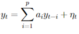
In the above equation, p represents the lag order, {η_t} is discrete white noise and a_i ∈ ℝ with a_p ≠ 0. Now, let us try to fit appropriate AR model to NIFTY daily returns and analyze the results. 

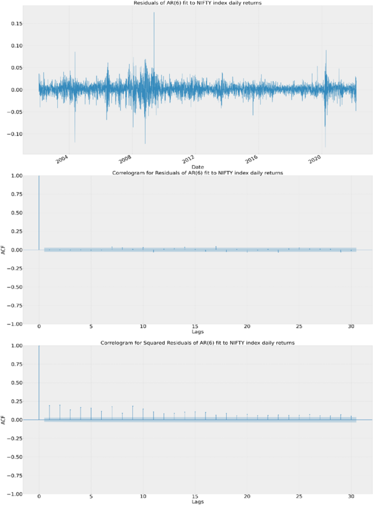
Looking at the above figure, we note some observations:

1. The middle graph shows insignificant autocorrelation at almost all lags except few (try to find the reason why there is significant autocorrelation at some lags and post it in comments). Insignificant autocorrelation here indicates that there is no serial correlation (autocorrelation) present in the series.
2. Last graph provides an evidence of AR model being not able to explain volatility clustering. Also, it is not able to explain black swan events. 

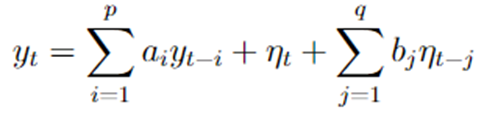
Next we have is Moving Average (MA) model:

Moving Average (MA) model: This model captures the unexpected (which are less likely to happen) events by taking a linear combination of past values of noise.

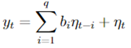
In the above equation, q represents the lag order, {η_t} is discrete white noise and b_i ∈ ℝ with b_q ≠ 0. Now, let us try to fit appropriate MA model to NIFTY daily returns and analyze the results.

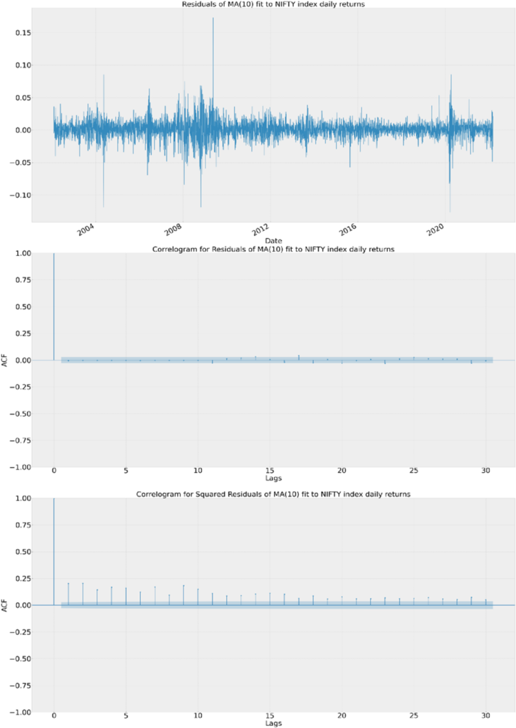
Again, we see insignificant autocorrelation in the middle graph but in the last graph, there is positive and significant autocorrelation in the squared residuals indicating that this model is not able to explain volatility clustering. 

Next in our store is Autoregressive Moving Average (ARMA) model:

ARMA model : It combines the above two models ( AR(p) and MA(q) ) to capture both their properties in a single model. One important use of ARMA model is that it usually requires less parameters than AR or MA model alone.

Autocorrelation graphs after fitting ARMA(1,2) model to NIFTY daily returns are shown below.

We conclude that although AR(p), MA(q) and ARMA(p,q) are able to explain no autocorrelation in the series but none of them could capture the volatility clustering effect. So, we need another type of models that can explain persistence in volatility. And here comes ARCH and GARCH in our picture. ARCH is Autoregressive Conditional Heteroskedasticity. We are already familiar with what autoregressive means. Then we move to Heteroskedasticity. Heteroskedasticity refers to the data with different variance (or standard deviation) when monitored over different time periods. Conditional Heteroskedasticity is when the varying variance is dependent on previous time periods. You should go back to the article on volatility clustering once and see the similarities in volatility clustering and conditional heteroskedasticity. Some people call conditional heteroskedasticity, a fancy (and statistical) term for volatility clustering. Now, let’s understand ARCH model.

ARCH model: The idea behind this is to model variance of the series as an autoregressive process to explain volatility clustering. Let’s try to understand it mathematically. 

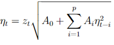
In the above equation, p represents the lag order, {z_t} is discrete white noise with mean 0 and variance 1, and A_i ∈ ℝ with A_p ≠ 0. Now we calculate variance of {η_t}. 

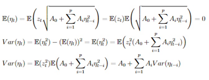
Let me try to explain the above calculations. In the first line, we are calculating mean of η_t using the fact that mean of z_t is 0 and z_t & η_(t-i) are independent. Using (η_t) = 0, we calculate Var(η_t) in the second and third line. Look closely at the last term and try to think of what it represents!!! It says that variance at time t is dependent on the previous variance terms and variance is directly related to volatility. This is what persistence of volatility means. So, mathematically ARCH model is able to explain volatility clustering. Now, Let us understand GARCH and check their autocorrelation graphs as well. 

GARCH model: After including autoregressive process in variance, the only thing left to add is the moving average which is the motivation for the GARCH model. 

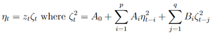
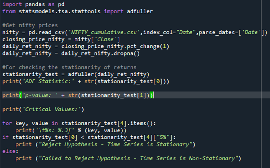
One thing should be kept in mind while fitting a GARCH model to a series that the series should be stationary. So, there are two ways in which GARCH model can be fitted to NIFTY daily returns. 

1. First step is to check if the given series is stationary or not using Augmented Dickey Fuller (ADF) test. If the series is stationary, then we can directly fit appropriate GARCH model to the given series.

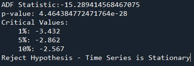
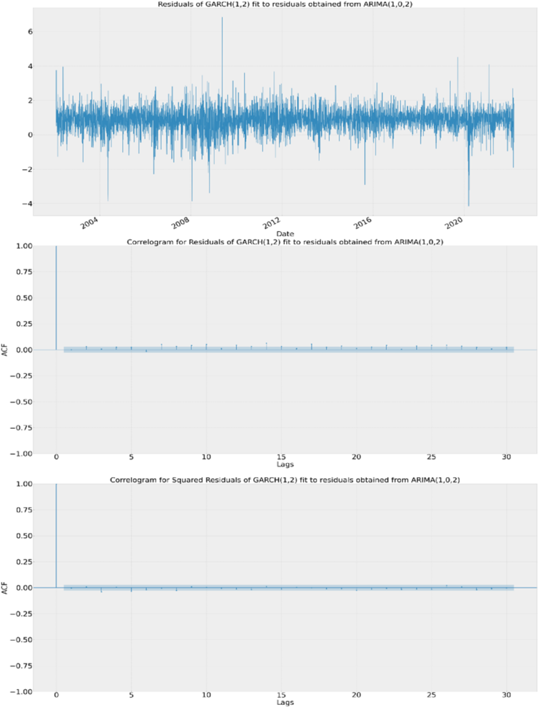
Now that we have verified that our series is stationary, it is time to check the autocorrelation graphs for the appropriate GARCH fitted model

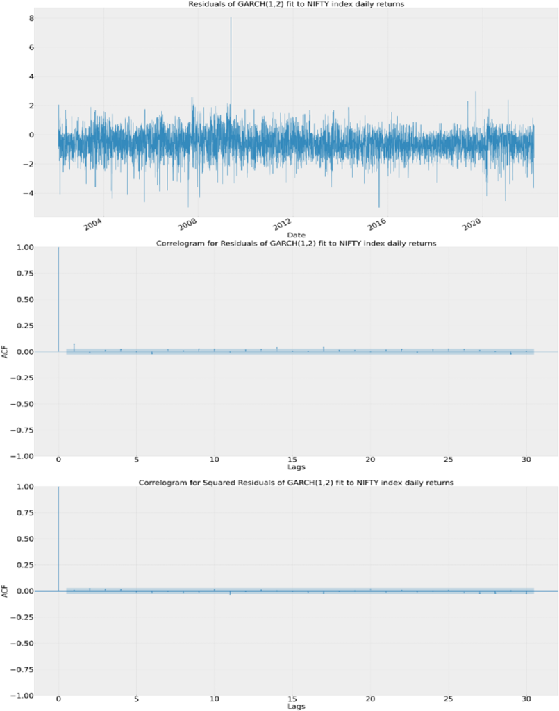
And finally, we are able to see insignificant autocorrelation in the squared residuals which shows that GARCH model has taken care of volatility clustering.

2. Suppose, In the first method the series turned out to be non-stationary, then what will you do?? This is where another variant of ARMA model known as Autoregressive Integrated Moving Average (ARIMA) model comes for our rescue. ARIMA model converts non-stationary series into stationary series by differencing. And then the residuals we get from ARIMA model are stationary and thus are fitted with appropriate GARCH model. 

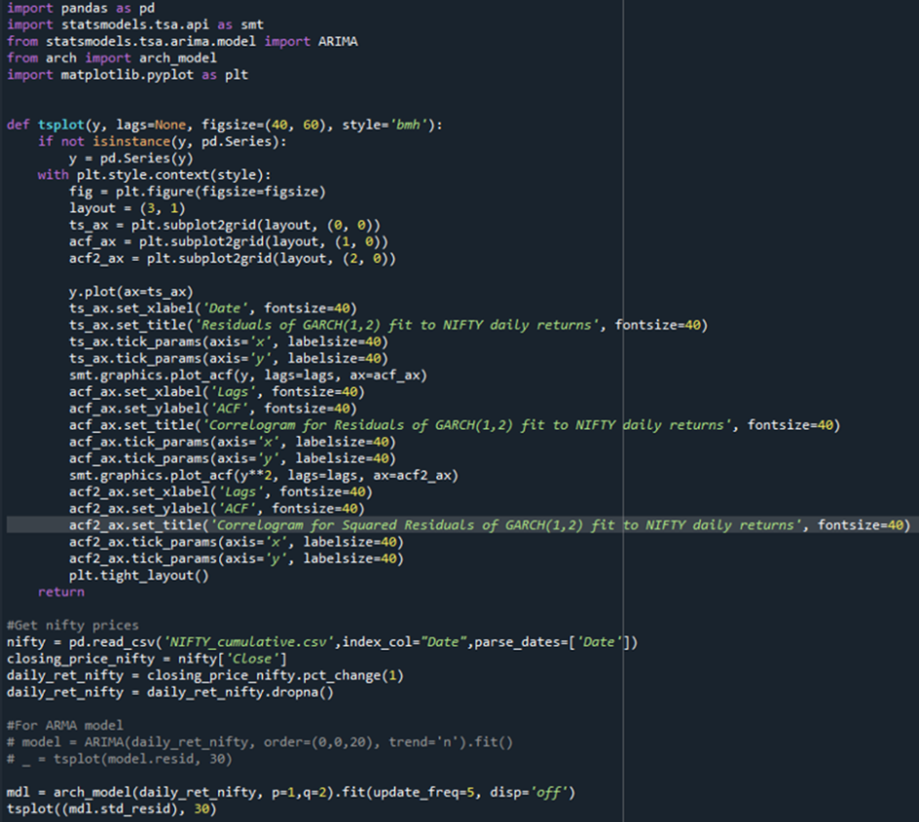
The following is used to plot the autocorrelation graphs shown in this article :

I have used the following references to write this article :

1. https://www.quantstart.com/articles/Generalised-Autoregressive-Conditional-Heteroskedasticity-GARCH-p-q-Models-for-Time-Series-Analysis/
2. https://analyticsindiamag.com/complete-guide-to-dickey-fuller-test-in-time-series-analysis/
3. http://www.blackarbs.com/blog/time-series-analysis-in-python-linear-models-to-garch/11/1/2016
4. https://towardsai.net/p/data-visualization/statistical-forecasting-for-time-series-data-part-5-armagarch-model-for-time-series-forecasting

Interested readers are encouraged to read more about how ARIMA + GARCH model is used in forecasting financial time series.