By Tushar Arora
Now that we have a basic understanding of Volatility and what it represents, let’s jump to the new concept: Volatility Clustering.
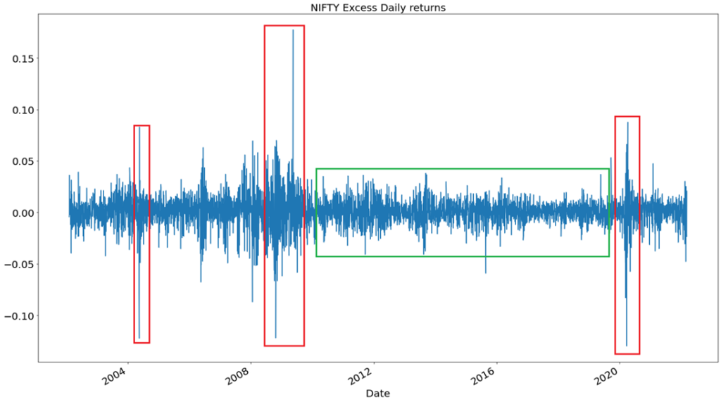
Again we come back to the same graph in which NIFTY returns are plotted. Notice that there are periods of high volatility and low volatility. We can’t find a period in the graph where we see fluctuations from low volatility to high volatility or high volatility to low volatility in a short amount of time. Why do you think this happens ? The answer lies in Volatility Clustering.
Volatility Clustering in most basic terms is persistence in volatility. What do we mean by persistence in volatility? It means that there will be periods of high volatility and periods of low volatility. Mandelbrot in his paper on “The Variation of Certain Speculative Prices” wrote a very nice observation which can be used to explain volatility clustering. The observation was “large changes are tend to be followed by large changes, of either sign, and small changes are tend to be followed by small changes.”
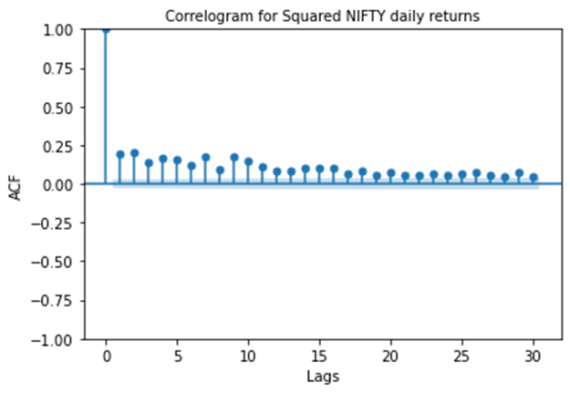
So, we understood volatility clustering and were able to explain it using the above graph. But understanding it pictorially is not enough, we have to find some mathematical evidence to support our observation. Let’s plot another graph.
What can we understand from this graph and how is it related with volatility clustering ? Let’s try to note some observations.
- It shows that cor((r_t)², (r_(t+lg))²) > 0 for all lg (lags) = 1, 2, … , 30 where r_t represents NIFTY daily return and cor represents Pearson correlation coefficient.
- cor((r_t)², (r_(t+lg))²) is significant (the value at every lag is above the light blue shaded region) for every lag.
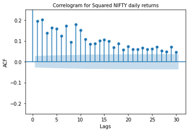
There is another observation which one can draw from the above graph. Try to post it in comments. How does these 2 observations relate to Volatility clustering? Think of what (r_t)² represent. Looking at NIFTY daily return series, it can be assumed that mean of the series is very close to zero. Then, (r_t)² will represent variance. Now, from the previous article we can see volatility coming in the picture. So, positive and significant correlation in (r_t)² & (r_(t+lg))² indicates that volatility at time t is positively correlated with volatility at time t+lg which provides the explanation for persistence of volatility.
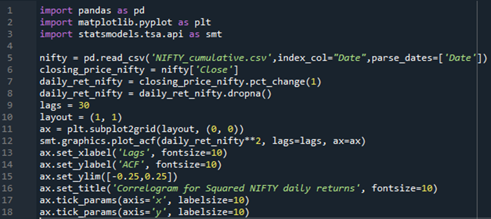
The following code has been used to plot “Significant autocorrelation in squared NIFTY daily returns at different lags” graph.
I have used the following references to write this article:
- https://en.wikipedia.org/wiki/Volatility_clustering#:~:text=In%20finance%2C%20volatility%20clustering%20refers,be%20followed%20by%20small%20changes.%22
- https://www.econometrics-with-r.org/16-4-volatility-clustering-and-autoregressive-conditional-heteroskedasticity.html
In the next article we will see how to model volatility clustering using GARCH models